Abstract
Why are dim-light sensing cells in eyes most sensitive to specific colors? There are explanations that delve into the detailed chemistry of how existing dim-light sensing cells work and explanations that chart the genetic lineage of their evolutionary development. However, might there be another level of approximation to an explanation that does not depend on these details? In this article the author hypothesizes that evolution has made dim-light sensing cells most sensitive to colors that make light detection minimally corrupted by the random noise inherent in the quantum mechanism of light absorption because this enhances the fitness of organisms. The author develops a theoretical physics implication of the hypothesis that begins at the quantum scale and applies statistics to zoom out to the biological scale; derives a mathematical expression for the absorbed light power signal-to-noise ratio (SNR)—where the source of noise is the quantum nature of the absorption process—as a function of the dominant color absorbed from sunlight; and ultimately predicts the colors that maximize this SNR in environments ranging from above sea level to the deep ocean. The difference between these predictions and observation is within the variability found between species in similarly lit environments, which range over about 5 nm. The author concludes that the hypothesis and theoretical physics implication is another level of approximation to a true explanation for why dim-light sensing cells of vertebrates in certain environments are most sensitive to specific colors of light, an explanation that complements those that depend on chemical details or genetic lineage.
I Introduction
Why are dim-light sensing cells in eyes most sensitive to specific colors? I hypothesize that the particular frequencies of peak absorption of photoreceptors of organisms can be influenced by evolutionary adaptation to the random noise that is superposed on light signals. This hypothesis implies that, among the various sources of noise, the inherent randomness of the quantum mechanics of light absorption can influence the evolution of dim-light photoreceptors in organisms because the associated light power absorption signal-to-noise ratio (SNR) can affect the evolutionary fitness of such organisms. This implication can be tested by determining whether this signal-to-noise ratio can be theoretically maximized and whether any photoreceptors approach this maximum.
Theoretical predictions can be compared with the experimental work of Shozo Yokoyama et al. [20], who deduced the genetic lineage of visual pigments in rod photoreceptor cells in retina (rhodopsins) in vertebrates. They engineered 11 ancestral rhodopsins and showed that those in early ancestors absorbed light maximally at a wavelength of about 501 nm, from which contemporary rhodopsins with variable peak absorption wavelengths of 480–525 nm evolved on at least 18 separate occasions, concluding that
based on considerations of ecology, life history, and s of rhodopsins, dim-light vision can be classified into biologically meaningful deep-sea, intermediate, surface, and red-shifted vision. The corresponding rhodopsins have s of 479–486, 491–496, 500–507, and 526 nm, respectively, establishing the units of possible selection. Consequently, it is possible that selective force may be able to differentiate even 4–5 nm of max differences of rhodopsins. [20]
Another historically interesting experiment to compare with theory was performed by J. K. Bowmaker and H. J. A. Dartnall [2], who concluded that the peak absorption wavelength of a sample of 9 rod cells from an eye of a man was nm. They went to great lengths to conduct this experiment.
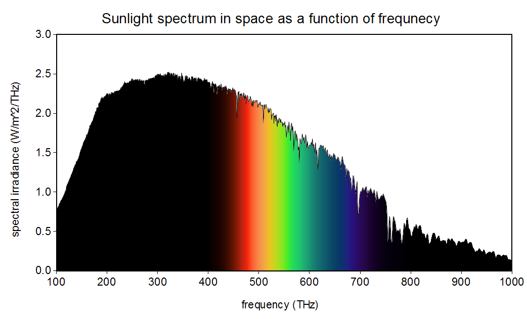
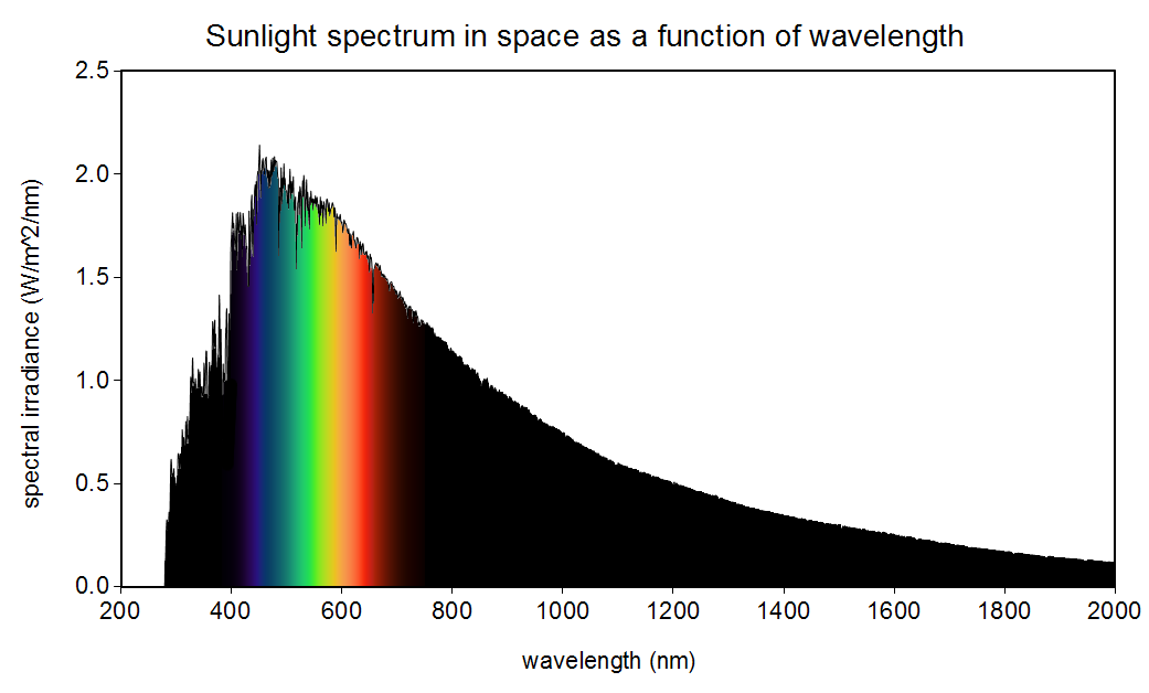
Yokoyama et al. refer to a popular alternative hypothesis to mine: that having dim-light sensing cells be most sensitive to wavelengths in a range where “the most abundant light falls” augments the fitness of organisms [20]. Bernard H. Soffer and David K. Lynch demonstrated how pervasive this hypothesis has been in the scientific literature and explain in detail why it is false, although they do not propose my hypothesis as an alternative [17]. In short, this popular hypothesis is false because the wavelength at the maximum of the spectral density as a function of wavelength and the frequency at the maximum of the spectral density as a function of frequency do not satisfy , the speed of light in vacuum. Figures 1 and 2 show these two functional forms of the spectral density of the Sun. Notice the apparent (illusory) concept of a range of wavelengths or frequencies where “the most abundant light falls” shifts between these two perspectives so that . My hypothesis, on the other hand, holds for both of these perspectives, as I will show.
I tested the theoretical implication of the hypothesis by (1) deriving a functional form of a signal-to-noise ratio (SNR) of light power absorption by an idealized photoreceptor (a classical system made up of many copies of a two-state quantum system) that depends on its peak absorption radial frequency and the spectral density of light illuminating the environment; (2) modeling how the Sun’s solar spectral density is attenuated at various depths of water; (3) maximizing the SNR by finding the zeros of its first derivative with respect to the peak absorption radial frequency; (4) comparing the predictions to experimental observations of rhodopsins in vertebrates that evolved in environments ranging from above sea-level to the deep ocean.
II Methods
II.1 Quantum mechanism of light absorption
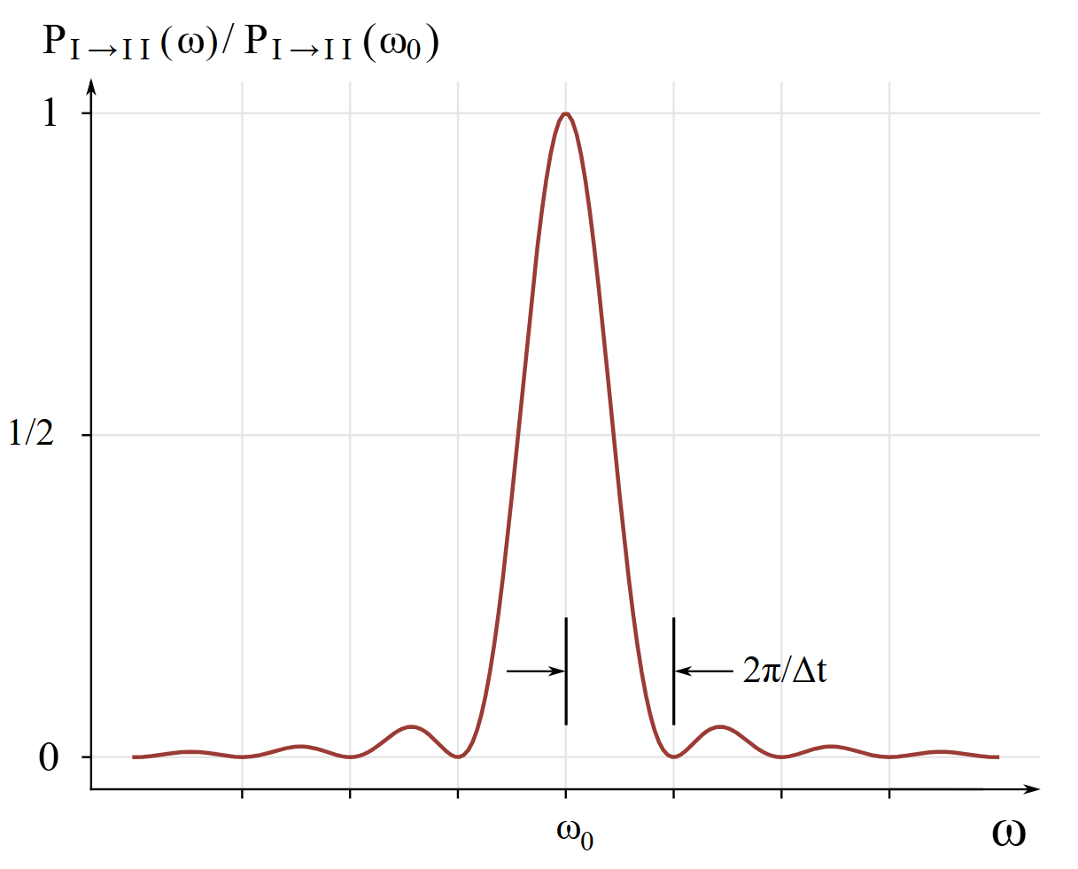
I begin where Feynman et al. explain off-resonance absorption of light by molecules in volume III chapter 9 section 5 of [6]. They consider the case that the amplitude of the electric field is small and also the period of time during which photon absorption may happen is small, so that , where is the resonant radial frequency of absorption for a molecule with an electric dipole moment. For this case, they derive the conditional probability that such a molecule will absorb a photon of monochromatic light over a time interval is
| (1) |
The absorbed photon’s energy raises the molecule’s energy from to , is the resonant absorption radial frequency, is the spectral radiance, is the time interval during which the absorption may happen, is the electric dipole moment of the molecule, is the speed of light in vacuum, is the reduced Planck constant, and is the vacuum permittivity. is plotted in Fig. 3 for a fixed and variable .
Unlike monochromatic light, sunlight has an intensity per unit frequency interval, covering a broad range which includes . Then the probability of absorption will become an integral over :
| (2) |
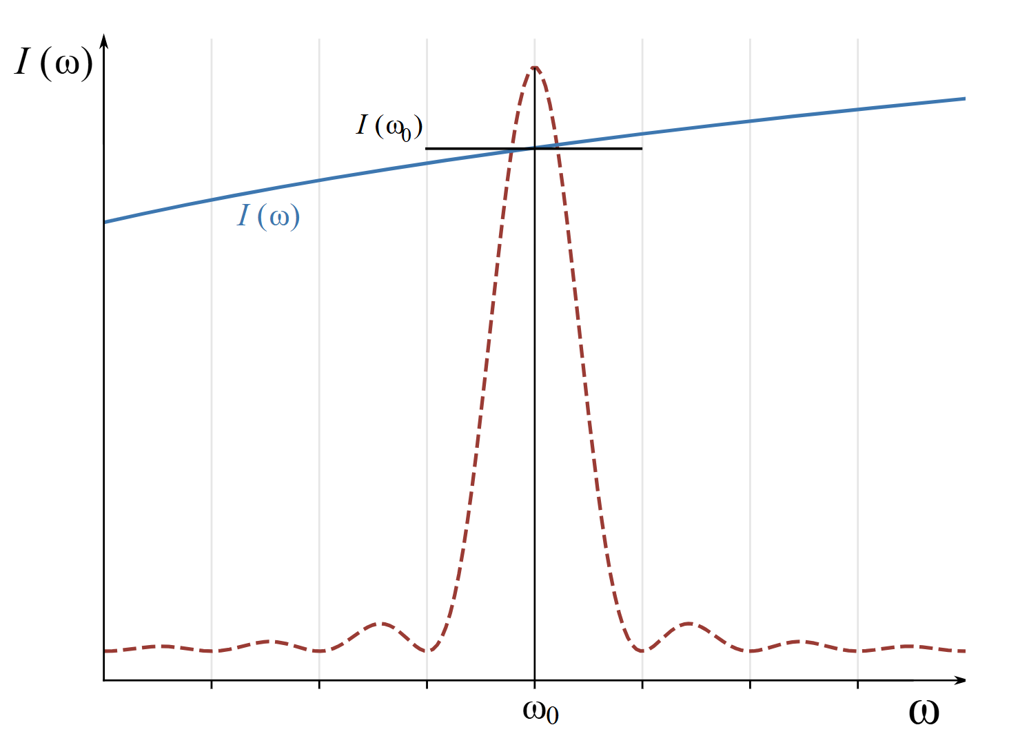
The solar spectral radiance varies much more slowly than the sharp resonance term. The two functions in the integral might appear as shown in Fig. 4. Since the solar spectral radiance is relatively constant over the relevant range of integration, it can be taken out of the integral.
| (3) |
The mean energy absorbed over a time interval is
| (4) |
or more explicitly,
| (5) |
This can be simplified by integrating over the interval where the probability peaks , making a change of variables , and approximating over the finite integration interval by its exact, closed form over to , which equals . The error of this approximation can be estimated by complex contour integration in the upper-half complex-plane along a semicircle of radius with an indentation around the origin. The approximation is exact to first order in the radius of the contour. The expression for the mean energy absorbed becomes
| (6) |
The mean energy absorbed over a time interval is inversely proportional to the half-width of the transition probability distribution’s central peak at . It is also directly proportional to the spectral radiance at the absorption peak.
The variance of the energy absorbed over a time interval is
| (7) |
or more explicitly,
| (8) |
Following much the same procedure as for the mean energy absorbed leads to the simplified form
| (9) |
Recall that this analysis began by considering the case where the electric field is small and also the period of time is small, so that , so the last term in square brackets is approximately equal to one, simplifying the variance to
| (10) |
The variance of the absorbed energy is directly proportional to the half-width of the transition probability distribution’s central peak at . It is also directly proportion to the solar spectral radiance at the absorption peak.
II.2 From quantum to biological scale
Now I will take the analysis from the quantum scale up to biological scale. After absorption events, the cumulative energy absorbed will reach a value of . The central limit theorem guarantees that the probability distribution of is Gaussian with a mean and variance
| (11) |
This is to be expected from a one-dimensional random walk, where the distance walked is analogous to the cumulative energy absorbed. This is why the noise I am considering here is generally referred to as ‘random-walk’ noise.
Viewed on energy-scales , looks like a continuous random process. At this energy-scale, the energy absorbed over the time interval , defined as , has a mean and variance of
| (12) |
So, by Eqs. 6 and 10, the mean energy absorbed and its variance over a time are
| (13) |
and
| (14) |
The mean power absorbed over a time interval is related to the mean energy absorbed by
| (15) |
and the absorption power variance is
| (16) |
The signal-to-noise ratio (SNR) of a Gaussian signal is the ratio of its mean squared and its variance (a unitless or dimensionless quantity). The SNR of the absorbed power is then
| (17) |
II.3 Maximizing the signal-to-noise ratio at and above sea level
The signal-to-noise ratio of light power absorption takes on its extreme values where its derivative with respect to is zero, which is where
| (18) |
The spectral density of the environment at and above sea level can be approximated by Planck’s law. This approximation ignores (1) the absorption spectrum of the Earth’s atmosphere and (2) the reflectance spectrum of the Moon, making no distinction between nocturnal and diurnal organisms. According to Planck’s distribution law, the spectral radiance of a black-body at a temperature is
| (19) |
where is the reduced Planck constant, is the speed of light in vacuum, and is the Boltzmann constant.
Using this functional form for , the left hand side of Eq. 18 is proportional up to a constant scalar multiple to
| (20) |
where . Writing the expression this way makes clear where the singularities of the derivative of are located: where the denominators and equal zero, which are at and . The zeros of Eq. 20 can be found by analyzing its Laurent series expansions about these singularities. These will be all of the zeros by the uniqueness theorem of Laurent series within their annular domain of convergence and by the fundamental theorem of algebra.
An analytic function has a zero of order at if
| (21) |
and .
Expanding the exponential functions about in terms of powers of , the right hand side of Eq. 20 can be written as
| (22) |
where
| (23) |
so , satisfying the condition .
Expanding the powers of and the exponential functions about in terms of powers of , the right hand side of Eq. 20 can be written as
| (24) |
where
| (25) |
so , satisfying the condition .
So, the zeros of the first derivative of with respect to peak absorption radial frequency are indeed at and ( and ). The higher-order (or general) derivative test can be used to determine whether either of these radial frequencies maximize .
Let all the derivatives of at be zero up to and including the -th derivative, but with the -th derivative being non-zero:
| (26) |
The higher-order derivative test guarantees that if is odd and , then is a local maximum; and if is odd and , then is a local minimum.
By Eqs. 22 and 24, the first non-zero derivative at the zeros is
| (27) |
Recalling that is the first derivative of near , the value of in the higher-order derivative test needs to be incremented by one more than is written in Eq. 27, and so is equal to 3, which is odd. So, according to the test, since by Eq. 23, is a local minimum; and since by Eq. 25, is a local maximum. These are the global minimum and maximum since these are the only zeros of the derivative of , as explained previously.
Converting back from to via , the analysis above shows that when the spectral density illuminating the environment at or above sea level is approximated by Planck’s law, the global maximum of the SNR is reached when a photoreceptor’s peak radial frequency .
II.4 Maximizing the signal-to-noise ratio below sea-level
How does the attenuation of light by water affect the prediction of the optimal peak absorption radial frequency for environments beneath the surface of bodies of water? The diffuse attenuation coefficient for irradiance is the apparent optical property that provides the most direct measure of the penetration of radiant energy in water,
| (28) |
where is the spectral irradiance at depth and is the irradiance at the surface.
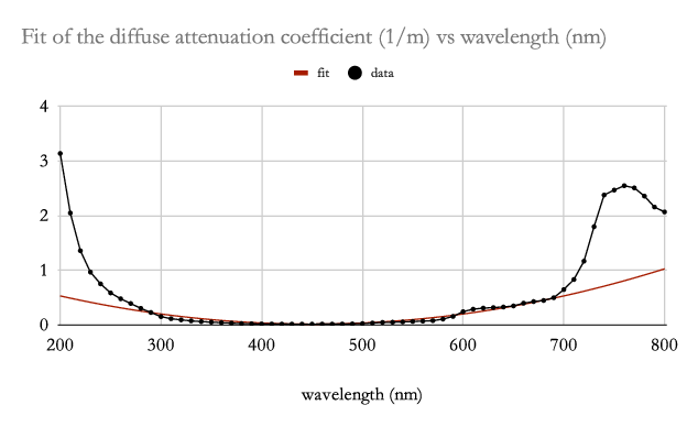
Raymond C. Smith and Karen S. Baker created a consistent set of data on the diffuse attenuation coefficient for irradiance of clear fresh- and salt-water environments for wavelengths in the range 200–800 nm [16]. Based on their data, the diffuse attenuation coefficient can be approximated in a neighborhood of its minimum value by a quadratic,
| (29) |
where the coefficient can be fit to their data. Such a fit is shown in Fig. 5. Fitting over all of their data, the coefficient of determination over the range 300–600 nm centered at 450 nm is 0.9961.
Using this approximation for and the attenuated spectral density in Eq. 28, the condition for maximizing the SNR in Eq. 18 is proportional up to a constant scalar multiple to
| (30) |
where
| (31) |
and is the scaled radial frequency where the diffuse attenuation coefficient is locally minimal.
Compare Eqs. 30 and 20. Notice the additional term in the square brackets that introduces a factor of .
Since the zeros of Eq. 30 are sought, it can be simplified by ignoring the exponential decay factor on the far right and grouping factors to emphasize the change in the expression going from the above-sea-level analysis to the below-sea-level analysis,
| (32) |
Notice the term in square brackets in Eq. 32. Going from the above-sea-level analysis to the below-sea-level analysis, this term changes according to
| (33) |
because at sea level . To see how this change affects the zero of Eq. 32, the right hand side can be factored into powers of to analyze it in the neighborhood of the zero of the above-sea-level analysis, . The expression becomes
| (34) |
Near , this expression can be truncated to the first power in , so the expression can be simplified to
| (35) |
The approximate change in the zero, , from to is characterized by
| (36) |
Comparing this form to Eq. 35, the approximate change in the zero when going from the above sea level to the below sea level analysis is
| (37) |
The approximate change in the zero has the limiting values (sea level) and (deep ocean). By the diffuse attenuation data of Smith and Baker [16], , so , which corresponds to a limiting shift of the peak absorption wavelength from nm at sea level to nm at extreme depths. Notice that the diffuse attenuation coefficient data of [16] is well approximated by a quadratic over this range as shown in Fig. 5 with a coefficient of determination of 0.9961, so the analysis is valid over the entire range of depths.
This predicted shift to shorter peak absorption wavelengths at lower and lower depths is consistent with what is observed in various species of fish [20]. Exceptions to this trend are deep sea fish that rely on bioluminescence to illuminate their environment, which have rhodopsins with peak absorption wavelengths of nm. Deep sea fish without bioluminescence have rhodopsins with peak absorption wavelengths in the range 479–486 nm, which are within the predicted range [20].
III Results and discussion
The result of the analysis above is that the signal-to-noise ratio of light power absorption, , of a photoreceptor when considering only the random-walk noise due to the quantum mechanism of light absorption is maximal when the peak absorption radial frequency of the photoreceptor is a zero of the function , where is the spectral density illuminating the environment as a function of radial frequency and depth of water. Translating from frequency to wavelength, the criteria is that the peak absorption wavelength is a zero of the function , where is the solar spectral density as a function of wavelength and depth of water.
This implication of the hypothesis gives compatible predictions when framed in terms of either wavelength () or frequency (), that is, , the speed of light in vacuum. The popular alternative hypothesis (that having dim-light sensing cells be most sensitive to wavelengths in a range where the most abundant light falls augments the fitness of organisms) does not give predictions that are compatible between these two framings.
The spectral density of the environment at and above sea level can be approximated by Planck’s law. This approximation ignores (1) the absorption spectrum of the Earth’s atmosphere and (2) the reflectance spectrum of the Moon, making no distinction between nocturnal and diurnal organisms. With this approximation, the theoretically predicted peak absorption radial frequency of organisms at and above sea-level is , where is the Boltzmann constant, is the effective black-body temperature of the environmental light source, and is the reduced Planck constant. Using the effective temperature of the Sun as K [12] in this relationship predicts the peak absorption radial frequency with the maximal to be , or equivalently, a frequency of THz, or a wavelength of nm.
This prediction is close to what has been measured for human rod cells by [2], nm, and for early rhodopsins in many vertebrates by [20], nm. The difference between this prediction and observation is within the variability found between rhodopsins of species in similarly lit environments, which range over about 5 nm [20].
Below sea level, the spectral density is diffusely attenuated as a function of wavelength (frequency). The attenuation shifts the predicted maximal peak absorption wavelength to shorter values at deeper depths below sea level, with a limiting value at extreme depths of about nm. This trend is consistent with what is observed in various species of fish that evolved at different depths and includes the range of peak absorption wavelength of deep sea fish that do not illuminate their environments with bioluminesence, 479–486 nm [20].
IV Conclusion
In conclusion, the experiments by [20], [2], and [16] verify the theoretical physics implication of the hypothesis that evolution makes dim-light sensing cells in eyes most sensitive to colors that maximize the light power absorption signal-to-noise ratio—where the noise is due to the inherent randomness of quantum mechanics—because having a greater signal-to-noise ratio enhances the fitness of organisms with such eyes.
This hypothesis supplants the popular hypothesis that evolution has made dim-light sensing cells most sensitive to colors with wavelengths (frequencies) in a range where the most abundant light falls because this augments the fitness of organisms.
This hypothesis supports the popular hypothesis that the evolution of the rod occurred very early in the history of life on Earth, since quantum mechanical randomness predates life on Earth. As stated in [9]:
Although the evolution of the rod and the duplex retina would have taken many generations, it must nevertheless have occurred very early: rods are present in every class of vertebrates including jawless cyclostomes, which split off from the rest of the vertebrates approximately 500 Ma. Moreover, the properties of lamprey rods and cones are very similar to those of rods and cones of gnathostomes. Recent experiments have shown, for example, that light adaptation in lamprey rods and cones is virtually indistinguishable from that in other vertebrates [10]. The early emergence of this new kind of ciliary photoreceptor together with the other retinal cells and synaptic pathways required for dim-light vision permitted the formation of the duplex retina, first postulated 150 years ago by Schultze [14], and now recognized to be a fundamental feature of vertebrate photodetection.
This hypothesis motivates investigation of the impact that other inherent sources of noise may have on the evolution of photoreceptors, along the lines of inquiry of [4, 13, 18, 19, 3]. Other questions come to mind:
-
•
Rod responses decay much more slowly than cones: exponential fits to the time course of decay give time constants about 10 times slower in rods than in cones [8]. The expression for the in Eq. 17 is linear with respect to , which can be interpreted as the sampling time of a photoreceptor. So, the increases with greater sampling time, or a slower time course of decay. Presumably, the responsiveness of an organism to its dynamic environment is a countervailing fitness pressure so there is a point of diminishing returns for a slower response. Might this explain the response speed of rods?
- •
-
•
Might cone peak absorption frequencies be influenced by other such sources of noise?
- •
Acknowledgements
I would like to thank Kenneth Cohen for his help.References
- [1] (2020) Quieting a noisy antenna reproduces photosynthetic light-harvesting spectra. Science 368 (6498), pp. 1490–1495. Cited by: 4th item.
- [2] (1980) Visual pigments of rods and cones in a human retina. J Physiol. 298, pp. 501–511. Cited by: §I, §III, §IV.
- [3] (1996) Light adaptation and reliability in blowfly photoreceptors. Int. J. Neural Syst. 7, pp. 437–444. Cited by: §IV.
- [4] (1943) The quantum character of light and its bearing upon threshold of vision, the differential sensitivity and visual acuity of the eye. Physica 10 (7), pp. 553–564. Cited by: §IV.
- [5] (2007) Evidence for wavelike energy transfer through quantum coherence in photosynthetic systems. Nature 446, pp. 782–786. Cited by: 4th item.
- [6] (2011) The feynman lectures on physics. Vol. III, Basic Books. External Links: Link Cited by: Figure 3, Figure 4, §II.1.
- [7] (1994) The primary steps of photosynthesis. Physics Today 47 (2). Cited by: 4th item.
- [8] (2015) Single-photon sensitivity of lamprey rods with cone-like outer segments. Curr. Biol. 25, pp. 484–487. Cited by: 1st item.
- [9] (2016) The evolution of rod photoreceptors. Phil. Trans. R. Soc. B 372. Cited by: §IV.
- [10] (2017) Evolution of adaptation in vertebrate photoreceptors. In Abstract 2687119, annual meeting of the Association for Research in Vision and Ophthalmology, Cited by: §IV.
- [11] (2007) The opsins of the vertebrate retina: insights from structural, biochemical, and evolutionary studies. Cell Mol. Life Sci 64, pp. 2917–2932. Cited by: 2nd item.
- [12] (2016) Nominal values for selected solar and planetary quantities: iau 2015 resultion b3. The Astronical Journal 152 (41). Cited by: §III.
- [13] (1948) The sensitivity performance of the human eye on an absolute scale. J Opt Soc Am 38 (2), pp. 196–208. Cited by: §IV.
- [14] (1866) Zur anatomie und physiologie der retina. Arch. Mikroskopische Anatomie 2, pp. 175–286. Cited by: §IV.
- [15] (2009) Evolution of opsins and phototransduction. Phil. Trans. R. Soc. B 364, pp. 2881–2895. Cited by: 2nd item.
- [16] (1981) Optical properties of the clearest natural waters (200–800 nm). Applied Optics 20 (2), pp. 177–184. Cited by: Figure 5, §II.4, §II.4, §IV.
- [17] (1999) Some paradoxes, errors, and resolutions concerning the spectral optimization of human vision. Am. J. Phys. 67 (11), pp. 946–953. Cited by: §I.
- [18] (1972) The molecular basis of visual excitation. In Nobel Lectures: Physiology or Medicine 1963–1970, Cited by: §IV.
- [19] (1994) Vibrationally coherent photochemistry in the femtosecond primary event of vision.. Science 266, pp. 422–424. Cited by: §IV.
- [20] (2008) Elucidation of phenotypic adaptations: molecular analyses of dim-light vision proteins in vertebrates. PNAS 105 (36), pp. 13480–13485. Cited by: §I, §I, §II.4, §III, §III, 2nd item, §IV.